Table of contents
Mathematical Equations in LaTeX
LaTeX provides a feature of special editing tool for scientific tool for math equations in LaTeX. In this
article, you will learn how to write basic equations and constructs in LaTeX, about aligning equations,
stretchable horizontal lines, operators and delimiters, fractions and binomials.
Mathematical modes
For writing math equations in LaTeX, there are two writing modes: the inline mode and the display mode. The
inline mode is used to write formulas that are part of the text and the display mode is used to write
expressions that are not part of the text and hence are put on different lines. The inline mode uses one of
the delimiters: \ ( \), $ $ or \begin{math} \end{math} and the display mode has two
versions: numbered and unnumbered. To print equations in display mode one these delimiters are used:
\[ \], $$ $$, \begin{displaymath} \end{displaymath} or \begin{equation}
\end{equation}.
How to write mathematical notations in LaTeX?
There are three ways to write a math equation in LaTeX and they are described as follows:
1. Inline: An inline expression occurs in the middle of the text. For producing an inline
expression, the math expression should be written between the dollar sign ($). For example, $E=mc^2 will
give E=mc^2.
2. Equation: Mathematical expressions that are given in a line are known as expressions.
These are basically placed on the centre of the page and the equations are important ones that deserve to be
highlighted. The inline expression shall be put in between \[ and \].
3. Display style: The command \displaystyle is used to get a full sized inline
expression.
Writing basic constructs of math in LaTeX
A formula is made up by combining various constructs. Some of them are explained below:
1. Arithmetic Operations:
-
Arithmetic equations are typed with a dollar sign. For example, $a + b$, $a - b$, $-a$, $a / b$, $a b$. There are different forms for multiplication and division that are $a \cdot b$, $a \times b$, $a \div b$.
-
Fractions are typed with the \frac command by putting the denominator and numerator with separate curly brackets.
-
The display style fraction inline command \dfrac can be used with the \tfrac environment for basically matrices so that the entries look small.
-
For subscripts and superscripts, we use ‘_’ and ‘^’ respectively. For example, a_{1},\ a_{i_{1}},\ a^{2},\ a^{b^{c}} will yield the result.
-
There is one symbol that can be automatically superscripted that is, '. For example, $f'(x)$ will yield and to get we input $f^{\prime 2}$.
-
For indicating dualspace, use the command ${}^{\dagger}$ where the {} means empty group.
-
The commands \sb and \sp are used for subscripts and superscripts respectively.
2. Binomial Coefficients:
-
Binomial coefficients are written with command \binom by putting the expression between curly brackets.
-
We can use the display style inline command \dbinom by using the \tbinom environment.
3. Ellipses:
-
There are two ellipses low or on the line ellipses and centered ellipses.
-
The low or on the line ellipses are types as F(x_{1}, x_{2}, \dots, x_{n}) and the centered ellipses are typed as x_{1} + x_{2} + \dots + x_{n}.
-
LaTeX gives \ldots command to distinguish between low and \bdots for centered ellipses.
The other variants for \dots command are \dotsc for an ellipse followed by comma, \dotsb for an ellipse
followed by a binary operation, \dotsm if followed by multiplication, \dotsi for an ellipse with integral
and \dotso for an “other” ellipse.
4. Integral:
-
In an integral math equation in LaTeX, the lower limit is taken as a subscript and the upper limit is taken as a superscript. For example, the code $\int\limits_{-\infty}^{\infty} e^{-x^{2}} \, dx = \sqrt{\pi}$ yields.
-
The commands \oint, \iint, \iiint and \idotsint yield and respectively.
-
For complicated bounds, we use \substack command or the subarray environment.
5. Roots:
-
The command \sqrt produces the square root. For example, $\sqrt{5}$ and $\sqrt{a + 2b + c^{2}}$ gives and respectively.
-
Can be typed using the expression $\sqrt[g]{5}$ and the position of ‘g’ can be adjusted by providing the additional commands: \leftroot moves ‘g’ left or right with negative argument and \uproot moves ‘g’ up or down with negative attribute.
Writing single equation
	\documentclass{article}
	\usepackage[utf8]{inputenc}
	\usepackage{amsmath}
	\begin{document}
	\begin{equation} \label{eqn}
	E = {mc^2}
	\end{equation}
 	 The equation \ref{eqn} states mass equivalence relationship.
	\end{document}
Output of the above code
Aligning Equations
We use the equation environment to wrap our equation or we can use equation if we want it to be numbered. The
environment split is used inside an equation environment to split the equation into smaller pieces which
will be aligned accordingly.
	\documentclass{article}
	\usepackage[utf8]{inputenc}
	\usepackage{amsmath}
	\begin{document}
	\begin{equation} \label{eq1}
	\begin{split}
	A & = \frac{\pi r^2}{2} \\
	 & = \frac{1}{2} \pi r^2
	\end{split}
	\end{equation}
	\end{document}
Output of the above code
Displaying long equations
The equations that utilise more than one line use multiline environment. We use a double backslash to set the
point where equation has to be broken. The first line is aligned to the left and the second line is aligned
to the right. We use * to determine whether the equation has to be numbered or not.
	\documentclass{article}
	\usepackage[utf8]{inputenc}
	\usepackage{amsmath}
	\begin{document}
	\begin{multline*}
	p(x) = x^8+x^7+x^6+x^5\\
	- x^4 - x^3 - x^2 - x
	\end{multline*}
	\end{document}
Output of the above code
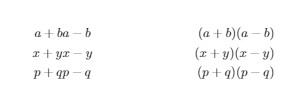
Aligning several equations
We use the align environment with * for determining whether the equation is numbered or not.
	\documentclass{article}
	\usepackage[utf8]{inputenc}
	\usepackage{amsmath}
	\begin{document}
	\begin{align*}
	a+b        &     a-b              &  (a+b)(a-b)\\
	x+y         &  x-y   &  (x+y)(x-y)\\
	p+q   &  p-q          &  (p+q)(p-q)
	\end{align*}
	\end{document}
Output of the above code
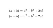
Grouping and Centering Equations
Math equation in LaTeX provides three stretchable lines/arrows that appear above or below the equation:
braces, bars and arrows. The \overbrace command places a brace above the expression (or
variables) and the command \underbrace places a brace below the expression. The command \overline
and \underline places a line above or below the expression. The command \overleftarrow
and \overrightarrow places an arrow above or below the expression. The expression has to be
written between curly brackets.
	\documentclass{article}
	\usepackage[utf8]{inputenc}
	\usepackage{amsmath}
	\begin{document}
	\begin{gather*}
	(a+b)=a^2+b^2+2ab \\
	(a-b)=a^2+b^2-2ab
	\end{gather*}
	\end{document}
Output of the above code
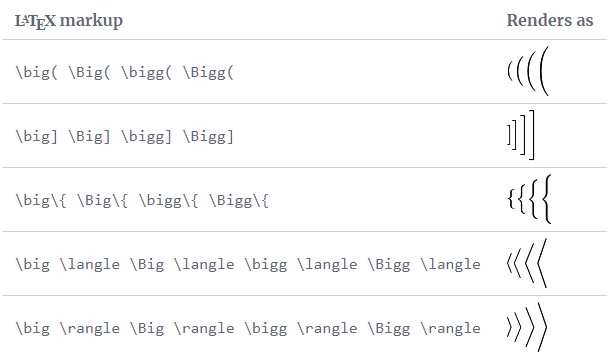
Parenthesis or Brackets
Parenthesis and brackets are very common in a mathematical equation. We can amend the size of a bracket in
math equations in LaTeX.
	\documentclass{article}
	\usepackage[utf8]{inputenc}
	\usepackage{amsmath}
	\begin{document}
	\[
	\left \{
	  \begin{tabular}{ccc}
	  1 & 5 & 8 \\
	  0 & 2 & 4 \\
	  3 & 3 & -8
	  \end{tabular}
	\right \}
	\]
	\end{document}
Output of the above code
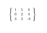
Size of the brackets can be changed as described below
Operators
There are various types of operators like trigonometrical functions, logarithms and others which are written
using special functions.
	\documentclass{article}
	\usepackage[utf8]{inputenc}
	\usepackage{amsmath}
	\begin{document}
	\[
	\sin^2(a)+\cos^2(a) = 1
	\]
	\end{document}
Output of the above code
The operators that take parameters are written in a special way. For example, in a limit equation, the limit declaration includes a subscript.
	\documentclass{article}
	\usepackage[utf8]{inputenc}
	\usepackage{amsmath}
	\begin{document}
	\[
	\lim_{h \rightarrow 0 } \frac{f(x+h)-f(x)}{h}
	\]
	 This operator changes when used alongside
	text \( \lim_{x \rightarrow h} (x-h) \).
	\end{document}
Output of the above code
The user can define or personalise his operator by using the command \DeclareMathOperator which takes two parameters, the first one is the name of the new operator and the second one is the text to be displayed. If the operator uses subscripts then the command \DeclareMathOperator* is used.
Fractions and Binomials
Fractions and binomial coefficients of math equations in LaTeX are written using the \frac and
\binom command respectively.
	\documentclass{article}
	\usepackage[utf8]{inputenc}
	\usepackage{amsmath}
	\begin{document}
	\[
	    \binom{n}{k} = \frac{n!}{k!(n-k)!}
	\]
	\end{document}
Output of the above code
We use the \frac command to display fractions. The expression between the first pair of brackets is the numerator and in the second is the denominator. The text size of the fraction changes according to the text near it. You can also set the text size of the fraction manually by using the command \displaystyle.
	\documentclass{article}
	\usepackage[utf8]{inputenc}
	\usepackage{amsmath}
	\begin{document}
	\[ f(x)=\frac{P(x)}{Q(x)} \ \ \textrm{and}
	\ \ f(x)=\textstyle\frac{P(x)}{Q(x)} \]
	\end{document}
Output of the above code
Fractions can be nested to obtain complex expressions. The command \cfrac displays nested fractions without changing the text size. An example of it is given below:
	\documentclass{article}
	\usepackage[utf8]{inputenc}
	\usepackage{amsmath}
	\begin{document}
	\[ \frac{1+\frac{a}{b}}{1+\frac{1}{1+\frac{1}{a}}} \]
	\end{document}
Output of the above code